Foreword
Have you ever wondered how babies and animals learn? How ChatGPT generates its texts? How DeepL translates texts? Well, part of it is due to SSL methods.
This article is the first part of the series around Self-Supervised Learning. No knowledge is required to understand the main message this article is trying to get across.
Nevertheless, since most of the methods presented above are based on Siamese networks, if you feel you need it, you can read our blog post on the subject beforehand.
The experimentations described in the article were carried out by building on the well-known library lightly by Susmelj et al. (2020).
Introduction
Over the past decades, we have witnessed a dramatic surge in data availability, thanks to new data formats beyond text (images, audio, videos, surveys, sensors, etc.), emerging technologies (data storage, social media, Internet of Things, data transfer, etc.), and data duplication. Drawing inferences from such big data using traditional techniques has been challenging. However, supervised learning techniques have become the go-to approaches for constructing predictive models with higher accuracy, surpassing human-level performance in recent years.
Despite the success of these approaches, they often depend on extensive labeled data. Labeling data can be a lengthy, laborious, tedious, and costly process compared to how humans approach learning, often making the deployment of ML systems cost-prohibitive. Therefore, the recurring question has been how to make inferences in a supervised learning setting with minimal labeled data. Current approaches to tackling this challenge rely on unsupervised and self-supervised learning techniques. Both self-supervised and unsupervised learning methods don't require labeled datasets, making them complementary techniques.
This article focuses on self-supervised techniques for classification tasks in computer vision. In the following sections, we delve into what self-supervised learning is, provide some literature on this burgeoning research topic, list self-supervised learning methods used in this article, describe experiments on public data, and finally, report results.
What is self-supervised learning?
Self-supervised learning (SSL) is a type of machine learning in which a model learns to represent and understand the underlying structure of data by making use of the inherent patterns and relationships within the data itself, rather than relying on explicit labels or annotations.
In SSL, the model is trained on a task that is automatically generated from the input data, such as predicting the missing parts of an image, predicting the next word in a sentence, or transforming an image into another modality like text or sound. By solving these tasks, the model learns to capture the underlying structure of the data and can generalize to new, unseen data.
The key to SSL is that it pre-trains the deep neural networks on large datasets, and then fine-tuned them for specific downstream tasks such as classification, object detection, and language modelling. It has been used to achieve state-of-the-art results on various tasks in computer vision, natural language processing, and speech recognition (see Section literature review below).
SSL techniques include but are not limited to:
1. Contrastive learning involves training a model to distinguish between similar and dissimilar examples. It learns to map similar examples closer together in a latent space while pushing dissimilar examples further apart.
2. Autoencoders train a model to encode an input into a compact latent representation and then decode it back into the original input. By minimizing the difference between the input and the reconstructed output, the model learns to capture the underlying structure of the data.
3. Generative model techniques train a model to generate new examples that are similar to the input data. Variational Autoencoders (VAEs) and Generative Adversarial Networks (GANs) are commonly used generative models in self-supervised learning.
4. Multitask learning techniques train a model on multiple related tasks simultaneously, leveraging the shared structure between the tasks to improve the model's ability to capture the underlying structure of the data.
5. Predictive coding by Millidge et al (2022) : This technique trains a model to predict the next frame in a video or the next word in a sentence, based on the previous frames or words. By doing so, the model learns to capture the temporal structure of the data.
6. Non-Contrastive Learning refers to techniques that do not rely on explicit comparisons between examples to learn representations. Instead, these methods use other types of learning signals to train the model.
Our primary focus here is on contrastive and non-contrastive methods. We will assess the performance of selected methods on various image datasets for classification tasks.
Literature review
The most comprehensive and well-organized review we have identified is the community-driven one hosted by Jason Ren. There, you will find the most relevant articles/presentations on this subject, categorized for easy navigation. His repository includes links to detailed blogs, to which we can add articles by blog from FAIR, Neptune.ai and v7labs.
Methods considered
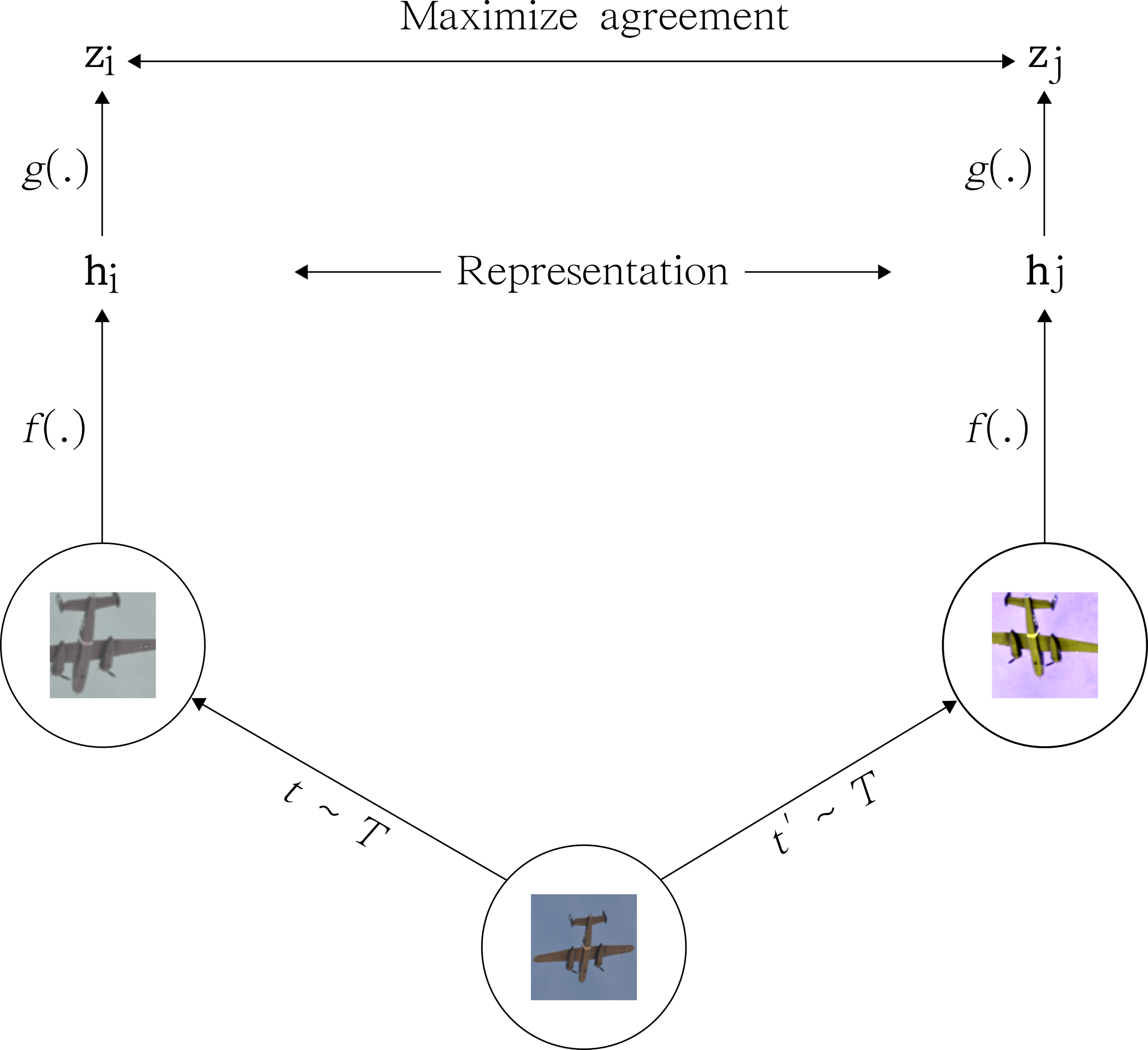
SimCLR (Simple Contrastive Learning of Representations) by Chen et al. (2020)
SimCLR learns representations by maximizing the agreement between different augmented views of the same image while minimizing the agreement between different images. Specifically, SimCLR uses a contrastive loss function that encourages representations of the same image to be close together in a high-dimensional embedding space, while pushing representations of different images further apart. The idea is that if two different views of the same image produce similar representations, these representations must capture useful and invariant features of the image (see Figure 1).
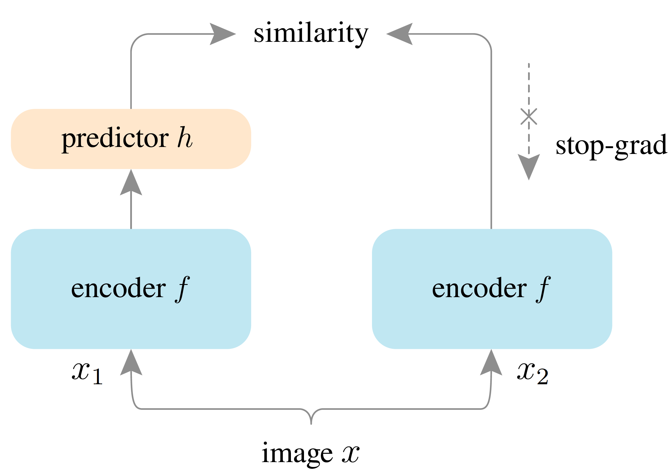
SimSiam (Exploring Simple Siamese Representation Learning) by Chen et He (2020)
Similar to SimCLR, SimSiam learns representations by maximizing the agreement between differently augmented views of the same image. However, unlike SimCLR, SimSiam omits the use of negative samples, meaning it does not compare representations of different images. Instead, SimSiam employs a Siamese network architecture with two identical branches with the same parameters. One branch generates a predicted representation of an image, while the other branch produces a randomly augmented version of the same image. The objective is to train the network to predict the augmented representation using only the other branch (see Figure 2).
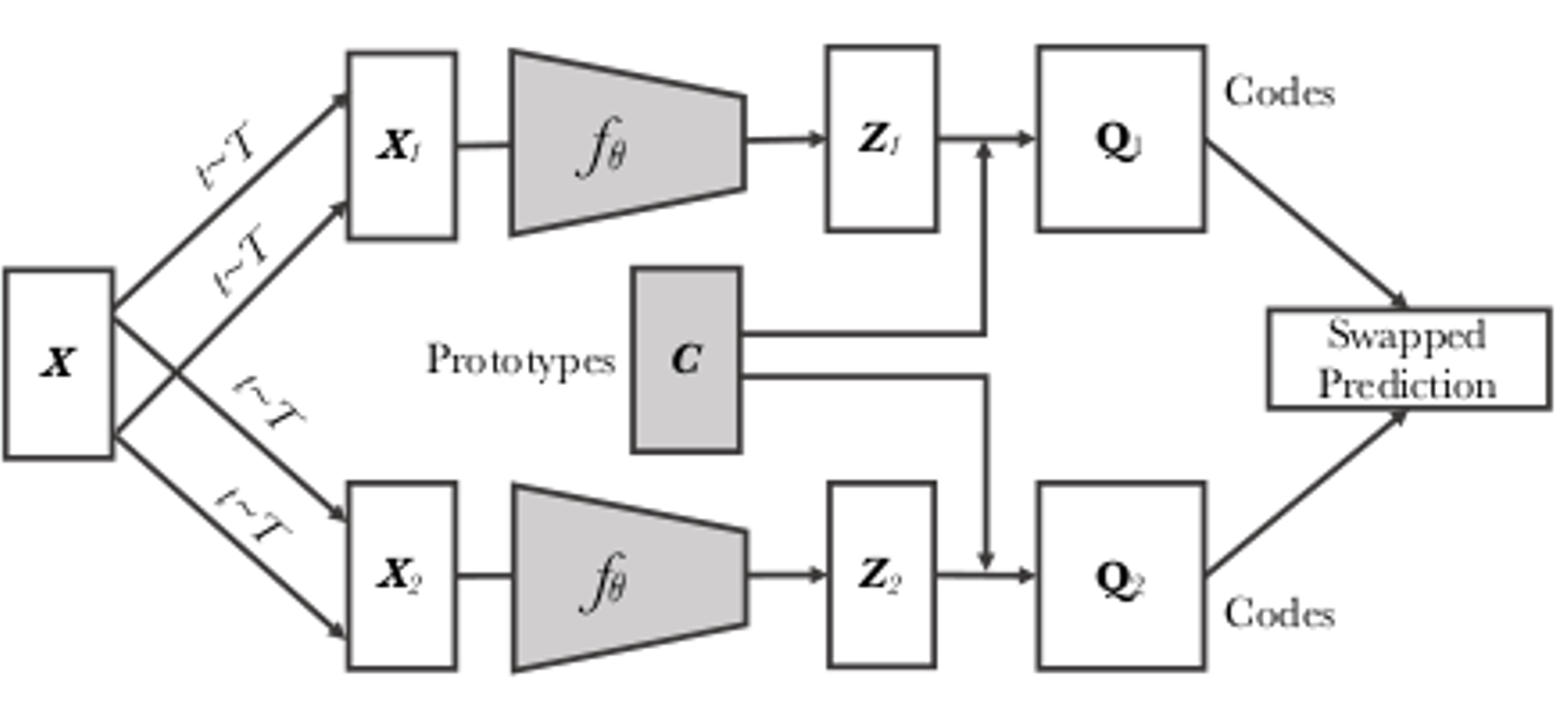
SWAV (Swapping Assignments between multiple Views of the same image) by Caron et al. (2020)
SWAV aims to learn representations that capture the semantic content of images. The method involves training a network to predict a set of learned "prototypes" for a given image. These prototypes are learned by clustering the representations of different augmented views of the same image. During training, the network is trained to predict which prototype corresponds to each view of the image, while also minimizing the distance between the representations of the views belonging to the same image (see Figure 3).
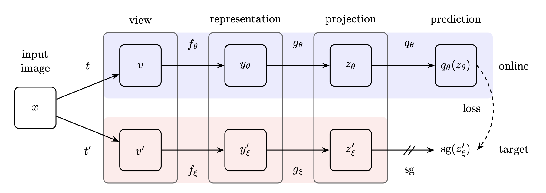
BYOL (Bootstrap Your Own Latent) by Grill et al. (2020)
BYOL involves training two copies of the same network to predict each other's outputs. One copy of the network, referred to as the 'online' network, is updated during training, while the other copy, known as the 'target' network, remains fixed. The online network is tasked with predicting the output of the target network, which, in turn, serves as a stable target for the online network. BYOL introduces a key innovation by employing a 'predictive coding' approach, where the online network is trained to predict a future representation of the target network. This methodology enables the network to learn representations that exhibit greater invariance to data augmentation compared to those acquired through contrastive learning methods (see to Figure 4).
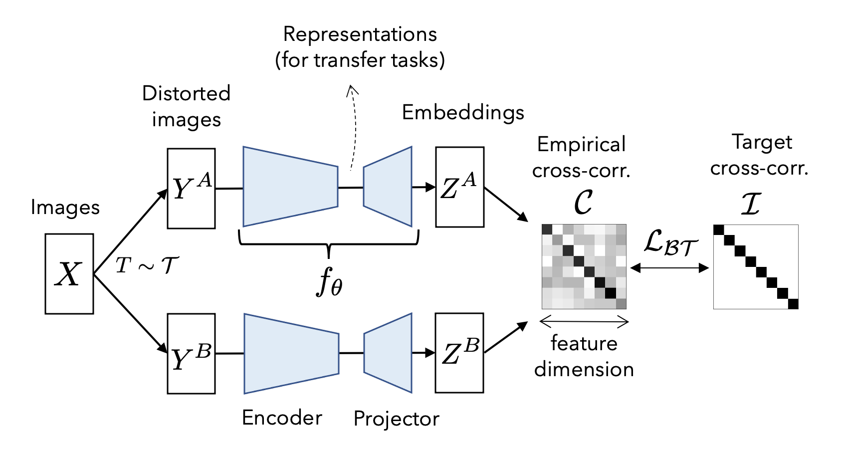
Barlow Twins by Zbontar et al. (2021)
Barlow Twins is based on the idea of maximizing the agreement between two randomly augmented views of the same data point while minimizing the agreement between different data points (see Figure 5). The underlying idea is that if two distinct views of the same data point yield similar representations, then these representations must encapsulate meaningful and invariant features of the data. To achieve this, Barlow Twins introduces a novel loss function designed to foster high correlation between the representations of the two views. Specifically, the Barlow Twins loss is a distance correlation loss that gauges the distinction between the cross-covariance matrix of the representations and the identity matrix.
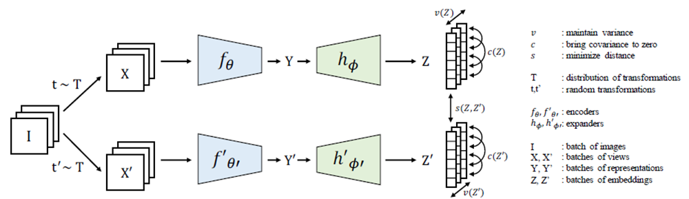
VICReg (“Variance-Invariance-Covariance Regularization”) by Bardes et al. (2021)
VICReg aims to improve the generalization performance of self-supervised models by encouraging them to capture the underlying structure of the data. It essentially learns feature representation by matching features that are close in the embedding space (see Figure 6). It does so by regularizing the model's feature representation using three types of statistical moments: variance, invariance, and covariance.
- Variance regularization encourages the model to produce features with low variance across different views of the same instance. This encourages the model to capture the intrinsic properties of the instance that are invariant across different views.
- Invariance regularization encourages the model to produce features that are invariant to certain transformations, such as rotations or translations. This encourages the model to capture the underlying structure of the data that is invariant to certain types of transformations.
- Covariance regularization encourages the model to capture the pairwise relationships between different features. This encourages the model to capture the dependencies and interactions between different parts of the data.
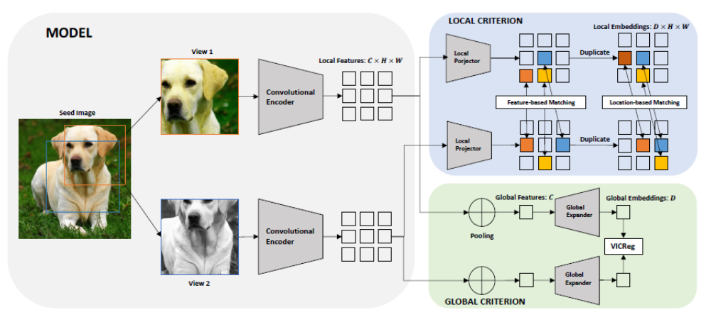
VICRegL by Bardes et al. (2022)
VICRegL is an extension of VICReg described above. In addition to learning global features, it learns to extract local visual features by matching features that are close in terms of locations in their original image (see Figure 7). It does that by using the regularization of VICReg in both the global and the local feature representation with the loss function described as a weighted sum of both local and feature-based losses. The weighted sum is governed by a scale factor $\alpha$ controlling the importance one wants to put on learning global rather than local representation. We refer the reader to the paper by Bardes et al. (2022) for details on how the loss function is derived.
Implementation details and results
We provide here the implementation details to reproduce these results. Here we built on the well-known library lightly to provide a much more flexible way of executing a classification task. The training pipelines are carefully designed and structured such that a new pipeline can be efficiently constructed without much code re-writing. This enables us to compare the effect of varying hyperparameters notably the parameters related to image transformation such as colour jitter, rotation angle, cropping etc on the performance of the SSL models.
For our benchmarks, we initially use a baseline transformation similar to that encoded in the library [lightly](https://github.com/lightly-ai/lightly) involving cropping, resizing, rotating, colour distortion (colour dropping, brightness, contrast, saturation and hue) and Gaussian blur. We then investigate the effect of four other transformations:
- the data augmentation methods used in SimCLR
- the transformation based on the horizontal and vertical flip (orthogonality)
- the LoRot-I transformation by Moon et al. (2022), i.e.draw and rotate a random area of the image
- the DCL transformation by Maaz et al. (2021), i.e. a deconstruction of the image using a confusion-by-regions mechanism.
We train the self-supervised models from scratch on various subsets of ImageNette by Howard (2019). These datasets include:
- ImageNette a subset of 10 easily classified classes from Imagenet (tench, English springer, cassette player, chain saw, church, French horn, garbage truck, gas pump, golf ball, parachute,
- ImageNette v2-160 (which is version 2 of ImageNette, where the distribution of training and by-validation samples is modified to 70%/30%, compared with 96%/4% in version 1. The number 160 indicates that the images are by size 160 by 160 pixels.)
- ImageWoof a subset of 10 dog breed classes from Imagenet, Australian terrier, border terrier, Samoyed, Beagle, Shih-Tzu, English foxhound, Rhodesian ridgeback, Dingo, Golden retriever, Old English sheepdog.
We also attempt to investigate the LoRot-I and DCL transformations on the NABirds by Van Horn et al. (2015) (North America Birds), a collection of 48,000 annotated photographs of the 550 species of birds that are commonly observed in North America) dataset.
It is important to note that while ImageNette and ImageNette v2-160 are easy to classify, ImageWoof and NABirds are not.
Since the VICRegL method requires both global and local transformations, we configure the parameters for global transformations as done for other methods, while those for local transformations follow the specifications outlined in the paper by by Bardes et al. (2022).
Four values of α are considered including 0.25, 0.5, 0.75 and 0.95 deciding the contribution of the global representation loss to the overall training loss. All experiments are implemented with a ResNet 18 backbone by He et al. (2015), 18-layer convolution NN utilizing skip connections or shortcuts to jump over some layers and each model is trained for 200 epochs with 256 batch size. It's important to note that we chose ResNet18 for its simplicity, and the experiment can be easily adapted to any backbone available in the PyTorch Image Models (timm) by Wightman (2019). In contrast to lightly, we include a linear classifier in the backbone instead of employing a KNN classifier on the test set. Our optimization protocol aligns with the guidelines outlined in the library lightly.
In total, 10 models are benchmarked on four different public data sets using five different transformations. The following tables show the test accuracy of each experiment realized on each SSL model. We include the executing time and the peak GPU usage for the ImageNette data set. Results are similar for the other data set. Overall, VICRegL and Barlow Twins seem to relatively outperform other models in terms of test accuracy. Except for the SimCLR and the orthogonality transformations, VICRegL models achieve similar accuracy to Barlow Twins with considerably less executing time as shown for the ImageNette data set. Also, we observe a lower peak GPU usage for VICRegL models compared to others. Interestingly, the test accuracy seems to be lower for results using the transformations that focus on some local parts of the images such as DCL and LoRot-I transformations. Conversely, the running time along with the peak GPU usage is lower for the latter transformations.
ImageNette
| Model | Batch size | Input size | Epochs | Test Accuracy Baseline | Test Accuracy SimClr | Test Accuracy Orthogonality | Test Accuracy LoRot-I | Test Accuracy DCL |
|---|---|---|---|---|---|---|---|---|
| BarlowTwins | 256 | 224 | 200 | 0.705 (123.8Min/11.1Go) | 0.772 (127.6Min/11.1Go) | 0.728 (132.3Min/11.0Go) | 0.675 (80.1Min/11.0Go) | 0.667 (90.1Min/11.0Go) |
| SimCLR | 256 | 224 | 200 | 0.679 (119.2Min/10.9GO) | 0.705 (135.8Min/11.8Go) | 0.682 (142.8Min/11.8Go) | 0.616 (64.8Min/11.8Go) | 0.626 (69.8Min/11.8Go) |
| SimSiam | 256 | 224 | 200 | 0.682 (119.1Min/11.9Go) | 0.691 (142.3Min/11.0Go) | 0.667 (142.3Min/12.7Go) | 0.611 (66.7Min/12.7Go) | 0.642 (66.3Min/12.7Go) |
| SwaV | 256 | 224 | 200 | 0.698 (120.5Min/11.9Go) | 0.693 (123.8Min/11.1Go) | 0.548 (143.1Min/12.7Go) | 0.626 (62.7Min/12.7Go) | 0.637 (61.2Min/12.7Go) |
| BYOL | 256 | 224 | 200 | 0.663 (122.4Min/13.3Go) | 0.659 (160.9Min/11.0Go) | 0.632 (164.2Min/14.2Go) | 0.610 (70.1Min/14.2Go) | 0.640 (70.0Min/14.2Go) |
| VICReg | 256 | 224 | 200 | 0.653 (121.0Min/11.8Go) | 0.718 (195.1Min/10.9GO) | 0.684 (196.6Min/12.7Go) | 0.613 (60.1Min/11.8Go) | 0.619 (59.7Min/11.8Go) |
| VICRegL, α=0.95 | 256 | 224 | 200 | 0.746 (60.0Min/7.7Go) | 0.744 (157.2Min/6.8Go) | 0.713 (160.8Min/8.6Go) | 0.702 (59.8Min/7.7Go) | 0.704 (59.8Min/7.7Go) |
| VICRegL, α=0.75 | 256 | 224 | 200 | 0.743 (59.1Min/7.7Go) | 0.744 (159.3Min/7.7Go) | 0.712 (171.3Min/8.6Go) | 0.700 (59.3Min/8.6Go) | 0.701 (56.1Min/8.6Go) |
| VICRegL, α=0.50 | 256 | 224 | 200 | 0.740 (58.2Min/7.7Go) | 0.742 (178.2Min/7.7Go) | 0.706 (188.5Min/8.6Go) | 0.697 (57.2Min/7.7Go) | 0.697 (54.2Min/7.7Go) |
| VICRegL, α=0.25 | 256 | 224 | 200 | 0.741 (58.1Min/7.7Go) | 0.742 (178.4Min/6.8Go) | 0.706 (198.5Min/8.6Go) | 0.695 (56.8Min/7.7Go) | 0.693 (53.8Min/7.7Go) |
ImageNette v2-160
| Model | Batch size | Input size | Epoch | Test Accuracy Baseline | Test Accuracy SimClr | Test Accuracy Orthogonality | Test Accuracy LoRot | Test Accuracy DCL |
|---|---|---|---|---|---|---|---|---|
| BarlowTwins | 256 | 224 | 200 | 0.763 | 0.677 | 0.653 | 0.649 | 0.618 |
| SimCLR | 256 | 224 | 200 | 0.685 | 0.665 | 0.594 | 0.588 | 0.621 |
| SimSiam | 256 | 224 | 200 | 0.678 | 0.663 | 0.592 | 0.590 | 0.652 |
| SwaV | 256 | 224 | 200 | 0.678 | 0.667 | 0.600 | 0.597 | 0.640 |
| BYOL | 256 | 224 | 200 | 0.661 | 0.636 | 0.587 | 0.589 | 0.632 |
| VICReg | 256 | 224 | 200 | 0.702 | 0.634 | 0.600 | 0.597 | 0.605 |
| VICRegL, α=0.95 | 256 | 224 | 200 | 0.724 | 0.723 | 0.698 | 0.691 | 0.692 |
| VICRegL, α=0.75 | 256 | 224 | 200 | 0.721 | 0.723 | 0.694 | 0.684 | 0.687 |
| VICRegL, α=0.50 | 256 | 224 | 200 | 0.709 | 0.710 | 0.691 | 0.680 | 0.682 |
| VICRegL, α=0.25 | 256 | 224 | 200 | 0.712 | 0.706 | 0.690 | 0.674 | 0.674 |
ImageWoof
| Model | Batch size | Input size | Epoch | Test Accuracy Baseline | Test Accuracy SimClr | Test Accuracy Orthogonality | Test Accuracy LoRot | Test Accuracy DCL |
|---|---|---|---|---|---|---|---|---|
| BarlowTwins | 256 | 224 | 200 | 0.507 | 0.455 | 0.460 | 0.448 | 0.416 |
| SimCLR | 256 | 224 | 200 | 0.457 | 0.423 | 0.403 | 0.396 | 0.397 |
| SimSiam | 256 | 224 | 200 | 0.437 | 0.420 | 0.393 | 0.393 | 0.401 |
| SwaV | 256 | 224 | 200 | 0.051 | 0.102 | 0.393 | 0.395 | 0.398 |
| BYOL | 256 | 224 | 200 | 0.436 | 0.401 | 0.392 | 0.399 | 0.413 |
| VICReg | 256 | 224 | 200 | 0.444 | 0.429 | 0.400 | 0.398 | 0.381 |
| VICRegL, α=0.95 | 256 | 224 | 200 | 0.464 | 0.446 | 0.443 | 0.428 | 0.430 |
| VICRegL, α=0.75 | 256 | 224 | 200 | 0.465 | 0.443 | 0.435 | 0.425 | 0.427 |
| VICRegL, α=0.50 | 256 | 224 | 200 | 0.466 | 0.443 | 0.435 | 0.423 | 0.420 |
| VICRegL, α=0.25 | 256 | 224 | 200 | 0.464 | 0.452 | 0.440 | 0.434 | 0.433 |
NABirds
| Model | Batch size | Input size | Epoch | Test Accuracy top 1% LoRot | Test Accuracy top 5% LoRot | Test Accuracy top 1% DCL | Test Accuracy top 5% DCL |
|---|---|---|---|---|---|---|---|
| BarlowTwins | 256 | 224 | 200 | 0.082 | 0.188554 | 0.093 | 0.214596 |
| SimCLR | 256 | 224 | 200 | 0.079 | 0.197335 | 0.097 | 0.237408 |
| SimSiam | 256 | 224 | 200 | 0.042 | 0.123549 | 0.061 | 0.161401 |
| SwaV | 256 | 224 | 200 | 0.073 | 0.193197 | 0.097 | 0.230342 |
| BYOL | 256 | 224 | 200 | 0.040 | 0.116786 | 0.059 | 0.165540 |
| VICReg | 256 | 224 | 200 | 0.083 | 0.188654 | 0.099 | 0.224589 |
| VICRegL α=0.95 | 256 | 224 | 200 | 0.155 | 0.334915 | 0.154 | 0.333603 |
| VICRegL α=0.75 | 256 | 224 | 200 | 0.155 | 0.332694 | 0.153 | 0.333199 |
| VICRegL α=0.50 | 256 | 224 | 200 | 0.150 | 0.326739 | 0.150 | 0.327344 |
| VICRegL α=0.25 | 256 | 224 | 200 | 0.144 | 0.314626 | 0.144 | 0.316443 |
Conclusion
- SSL in computer vision refers to making a computer learn the visual word with minimal human supervision.
- The choice of data augmentation is key to improving classification in computer vision problems.
- Accounting for local and global features during learning by using VICRegL model seems to give the best tradeoff between accuracy and computer capability for improving classification accuracy.
- Doing only pure SSL using LoRot-I and DCL transformations does not outperform traditional transformations.
- Future work on extending the scope of this work will be carried out e.g. using different backbones, more epochs etc. especially on ImageWoof and NABirds datasets.
- In the next article, we will measure the effectiveness of using the transformation as SSL pretext task as in Maaz et al. (2021).
References
- Predictive Coding: Towards a Future of Deep Learning beyond Backpropagation? by Millidge et al (2022),
- A Simple Framework for Contrastive Learning of Visual Representations by Chen et al. (2020),
- Exploring Simple Siamese Representation Learning by Chen et al. (2020),
- Exploring Simple Siamese Representation Learning by Chen et He (2020),
- Unsupervised Learning of Visual Features by Contrasting Cluster Assignments by Caron et al. (2020),
- Bootstrap Your Own Latent: A New Approach to Self-Supervised Learning by Grill et al. (2020),
- Barlow Twins: Self-Supervised Learning via Redundancy Reduction by Zbontar et al. (2021),
- VICReg: Variance-Invariance-Covariance Regularization for Self-Supervised Learning by Bardes et al. (2021),
- VICRegL: Self-Supervised Learning of Local Visual Features by Bardes et al. (2022),
- Tailoring Self-Supervision for Supervised Learning by Moon et al. (2022),
- Self-Supervised Learning for Fine-Grained Visual Categorization by Maaz et al. (2021),
- ImageNette by Howard (2019),
- Building a Bird Recognition App and Large Scale Dataset With Citizen Scientists: The Fine Print in Fine-Grained Dataset Collection by Van Horn et al. (2015),
- Deep Residual Learning for Image Recognition by He et al. (2015),
- PyTorch Image Models (timm) by Wightman (2019)